Meta-analysis

Meta-analysis and models to predict disease transmission in livestock

Location

Living Earth Collaborative Center for Biodiversity Working Group
St. Louis, USA

People

Amanda Koltz (co-organizer), Washington University in St. Louis, USA
Rachel Penczkowski (co-organizer), Washington University in St. Louis, USA
Sharon Deem (co-organizer), Institute for Conservation Medicine, St. Louis Zoo, USA
Vanessa Ezenwa (co-organizer), University of Georgia, USA
Susan Kutz, University of Calgary, Canada
Brandon Barton, Mississippi State University, USA
Zoe Johnson, Mississippi State University, USA
Aimee Classen, University of Vermont, USA
J. Trevor Vannatta, Purdue University, USA
Matt Malishev, Emory University, USA
David Civitello, Emory University, USA
Daniel Preston, University of Wisconsin-Madison, USA
Maris Brenn-White, St. Louis Zoo, USA

Tasks

Developed disease transmission models to predict parasite burden on wild animals and livestock
Built a keyword query bot for scraping web search data based on user search engine results (meta-analysis)
Built a meta-analysis text mining bot for scraping PDF files for user-defined data (meta-analysis)

Outcomes

Research

Ezenwa VO, Civitello DJ, Barton BT^, Becker DJ^, Brenn-White M^, Classen AT^, Deem SL^, Johnson ZE^, Kutz S^, Malishev M^, Penczykowski RM^, Preston DL^, Vannatta JT^ & Koltz AM (2020) Infectious diseases, livestock, and climate: a vicious cycle? Trends in Ecology and Evolution. https://doi.org/10.1016/j.tree.2020.08.012.

Software and models

Nutrient Quota Host-Parasite (NQHP) model

Tic-Tac-Toe spatial Nutrient Resource Susceptible Infected (NRSI) model

Keyword query bot

Data scraper bot

Media

Climate change has a cow and worm problem, The Verge, Oct 7, 2020.

Sicker livestock may increase climate woes, The Source, Washington University, Oct 7, 2020.

Example outputs

Nutrient Quota Host-Parasite (NQHP) model

Gut parasite disease transmission model tracking nutrient, biomass (resources), susceptible and infected host, and parasite densities with explicit nutrient exchange and recycling.

State variables (units = biomass)
N = nutrients in the landscape (biomass)
R = food in the landscape (food biomass)
QR = nutrient quota in food source (nutrient/carbon ratio). QF⋅ is total nutrients in food.
H = host consumer population (host biomass)
QH = nutrient quota in hosts (nutrient/carbon ratio)
P = parasite population (within-host parasite biomass)

Parameters
α = virulence
dH = death rate of hosts
dP = death rate of parasites
l = nutrient loss
mF = maximum food biomass
mH maximum host biomass
μM = maximum uptake rate of biomass
F = carbon biomass in food biomass
QR = nutrient to carbon (N/C) ratio in food biomass, so that QR⋅R is the nutrient level in food biomass
Recycling = e⋅QF⋅f⋅F⋅H

Nutrient growth (biomass)

Food growth (biomass)

Nutrient quota of food source

Host population growth (host biomass)

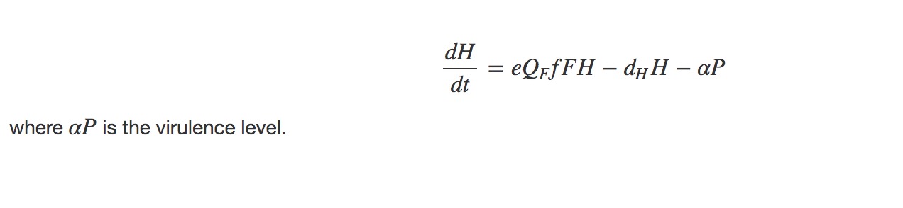
Nutrient quota in hosts (nutrient/carbon ratio)

Parasite population (within-host parasite biomass)

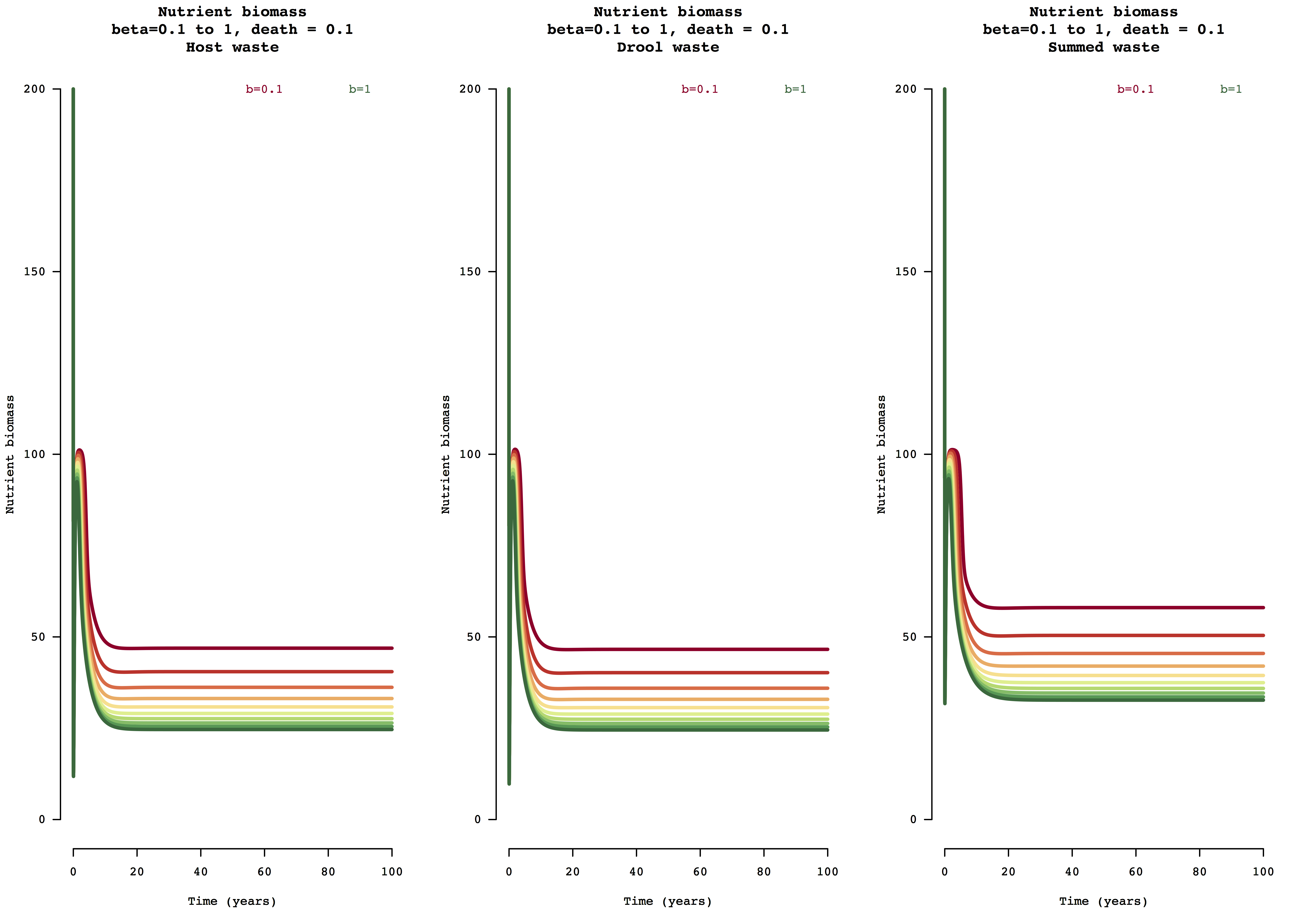
Figure 1. Example model output for nutrient (biomass) change over 100 years for the host waste, drool waste, and summed waste resource uptake and nutrient leaching modes of susceptible and infected host populations for beta transmission range [0,1].

Link to project page.

Tic-Tac-Toe spatial Nutrient Plants Susceptible Infected (NPSI) model

Consumer-resource disease transmission model of parasite loading on nutrient cycling in ecosystems as a spatial individual-based model of resources, host populations, and disease vector populations.

The project aims to predict how resource biomass uptake and release by infected and non-infected host populations varies under a disease mosaic landscape. Disease patches in the landscape are driven by feedback between modes and rates of disease transmission and costs of parasite transmission rates and nutrient deposit in space and time.

Link to project page.

Keyword query bot

The bot reads a .txt file containing literature entries resulting from a keyword search term query similar to a Web of Science database search. It then converts this file into a readable .csv file with each row as separate data, in this case, research articles. Using user-defined keyword search terms, it then scrapes the .csv file and returns a new file saved to the user’s local hard drive with the final data entries containing the user-defined search terms. Users can define what part of the article they want to search, e.g. Title, Author, Abstract, etc.

Download the instructions for running the bot in R
Download the model file (right click here and ‘Save link as’)
Run the model in R. The final outputs will save to your local directory.

keyword_final.csv
keyword_final_isolated.csv

Keyword query bot R code

Required files:

LEC100testrecords.txt
search_term_inputs.txt
article_col_names.txt
lec_keyword_search.R

Load packages and set working directory.

##########################################################################

# load packages (run once) ------------------------------------------------

install.packages("pacman")
require(pacman)
p_load(dplyr,purrr,readr)

# user inputs -------------------------------------------------------------

# set working dir
setwd("your working dir")

Choose whether to search the Title or the Abstract for the keywords and what article data you want returned, e.g. year of publication, the entire abstract, etc.

# Step 1 ----------------------------------------------------------------------

# Enter either Title or Abstract to search for the keywords
extract1 <- "Title" 

# Step 2 ------------------------------------------------------------------

# Now enter what data you want to get out of the final results
# For example, if you want to know what year in which the resulting papers were published,
# type in "Year"
# use any search term you specified in the search_terms_input file
extract2 <- "Year"

Open the search_term_inputs.txt file with a standard text editor and type in the following information.

First line
Your working directory where this document and the associated files are located. e.g.

/User/documents/models

Second line
Your search terms, separated by a comma. Spaces and lower/upper cases are OK too. For example, if you want to search for the following terms:

evidence
human
africa

You would type in the following:

evidence, human, africa

Third line
Enter the data entry you want to run the keyword search terms on from the below list. Note, case sensitive.

Primary entries:
Abstract
Author
Title
Year

Other possible entries:
BCI
CorrAuthor
ISSN
Issue
Journal
Link
Pages
PubDate
Volume

Fourth line (optional)
You can also enter what data you want to isolate from the final results to save as a separate file. For example, if you want to know just the year in which the selected papers were published, type in Year. Otherwise, leave blank.

Save the search_term_inputs.txt file and run the rest of the R code.

##########################################################################

# run rest of code from here ----------------------------------------------
# read in file ----------------------------------------------------------

fh <- "LEC100testrecords.txt"
anomalies <- 1 # save csv file of entries that contain the term 'Go to ISI' instead of article title 

ww <- readLines("search_term_inputs.txt") # set working dir
wd <- setwd(ww[1]) 
tt <- read.delim(paste0(wd,"/",fh),header=T,sep="\t")
tt %>% str
# set column names for df from file
df_colnames <- read.delim("article_col_names.txt",header=F,strip.white = T,sep=",",colClasses = "character")[1,] %>% as.character
colnames(tt) <- df_colnames

# view structure of data frame
tt %>% str
# randomly sample entries to see if contents align with the above col names
tt[sample(126,1),]

# key terms ---------------------------------------------------------------

keyterms <- read.delim("search_term_inputs.txt",header=F,skip=1,strip.white = T,sep=",",colClasses = "character")[1,] %>% as.character
keyterms <- keyterms %>% as.character ; keyterms_neat <- keyterms
keyterms <- paste(keyterms,collapse="|"); keyterms_neat # combine all the search terms 

final <- tt[grep(keyterms, tt[,extract1], ignore.case = T),] #
length(final[,extract1]) # get number of results
tt[final[,extract1],extract1] # show raw outputs 

### Remove NA columns  
rm_na <- grep("NA", names(tt), ignore.case = F)
final[,colnames(final[,rm_na])] <- list(NULL)

# extract isolated data col
ww <- as.list(ww); names(ww) <- ww
col_final <- ww[extract2] %>% as.character()
if(col_final!=""){final[,col_final]} # return as vector

# remove duplicate entries
final <- unique(final)

## Save output to file  
fho <- "keyword_final.csv"
write_csv(final,paste0(wd,"/",fho))

## Save isolated results data to file  
# final[col_final] # return as data frame column    
if(col_final!=""){
  final_isolated <- final[,col_final] # return as vector
  final_isolated <- as.data.frame(final_isolated); colnames(final_isolated) <- col_final
  fho_iso <- "keyword_final_isolated.csv"
  write.csv(final_isolated,paste0(wd,"/",fho_iso))
  cat(rep("\n",2),"Your results are saved as\n\n",fho_iso,"\n\n in","\"",wd,"\"","\n\n showing just",col_final,"data",rep("\n",2))
}

## Anomalies
### Here are the entries that contain the default term "<Go to ISI>" in the title column from the original data 
if(anomalies==1){
  gti <- "<Go to ISI>"
  search_func_gti <- grep(gti, tt[,"Title"], ignore.case = T)
  final_gti <- tt[search_func_gti,] #
  length(final_gti[,"Title"]) # get number of results
  tt[final_gti[,"Title"],"Title"] # confirm against raw data
  cat("Rows from original data where entries occur:\n",search_func_gti) # rows from original data where entries occur

  ### Remove NA columns  
  rm_na <- grep("NA", names(tt), ignore.case = F)
  final_gti[,colnames(final_gti[,rm_na])] <- list(NULL)
  
  ### Save anomalies to file
  fho_isi <- "keyword_final_anomalies.csv" # save these anomalies to local dir
  write.csv(final_gti,paste0(wd,"/",fho_isi))
  cat(rep("\n",2),"Your results are saved as\n\n",fho_isi,"\n\n in","\"",wd,"\"",rep("\n",2))
}

# final 
cat(rep("\n",2),"Your results are saved as\n\n",fho,"\n\n in","\"",wd,"\"","\n\n using the following search terms:\n\n",keyterms_neat,rep("\n",2),
"Total papers when searching",col2search,":",length(final[,col2search]))

The two files will be saved to your local working directory:

keyword_final.csv
keyword_final_isolated.csv

Results

Input: Snippet of raw data from default Web of Science keyword search query.

H. Ebedes	1975	THE CAPTURE AND TRANSLOCATION OF GEMSBOK ORYX GAZELLA-GAZELLA IN THE NAMIB DESERT WITH THE AID OF FENTANYL ETORPHINE AND TRANQUILIZERS		Journal of the South African Veterinary Association			46		4	359-362								THE CAPTURE AND TRANSLOCATION OF GEMSBOK ORYX GAZELLA-GAZELLA IN THE NAMIB DESERT WITH THE AID OF FENTANYL ETORPHINE AND TRANQUILIZERS		0038-2809												BCI:BCI197763001378				"Gemsbok (23) in the Namib Desert were captured with combinations of fentanyl or etorphine hydrochloride, hyoscine hydrobromide and tranquilizers such as axaperione, SU-9064 [methyl 18-epereserpate methyl ether hydrochloride], triflupromazine hydrochloride and acetylpromazine maleate. Fentanyl, a new immobilizing compound proved to be safe and effective for gemsbok. The gemsbok were chased on the interdune plains and darted from a Land Rover with the Palmer powder-charge Cap-Chur gun. A 6-seater helicopter was used on a trial basis to dart gemsbok but it is suggested that a small more maneuvrable helicopter be used for further operations. All the gemsbok were transported under narcosis from the capture area to an enclosure. Chlorpromazine hydrochloride was injected into the captured gemsbok to sedate them in their new confined environment. Tranquilizers such as chlorpromazine hydrochloride, acetylpromazine maleate and a new tranquilizer SU-9064 were used to sedate the animals during long distance transportation in crates. This prevented the animals from injuring themselves and damaging the crates. For the 1st time in South West Africa wild animals were transported by air. A journey by road which under normal circumstances would have taken over 40 h was completed in less than 9 h by air. There were no losses during transportation and only 2 gemsbok were injured during the translocation operation."			<Go to ISI>://BCI:BCI197763001378
"K. A. Durham, R. E. Corstvet and J. A. Hair"	1976	APPLICATION OF FLUORESCENT ANTIBODY TECHNIQUE TO DETERMINE INFECTIVITY RATES OF AMBLYOMMA-AMERICANUM ACARINA IXODIDAE SALIVARY GLANDS AND ORAL SECRETIONS BY THEILERIA-CERVI PIROPLASMORIDA THEILERIIDAE		Journal of Parasitology			62		6	1000-1002								APPLICATION OF FLUORESCENT ANTIBODY TECHNIQUE TO DETERMINE INFECTIVITY RATES OF AMBLYOMMA-AMERICANUM ACARINA IXODIDAE SALIVARY GLANDS AND ORAL SECRETIONS BY THEILERIA-CERVI PIROPLASMORIDA THEILERIIDAE		0022-3395		

Output: Queried data based on user search terms (truncated).

Author	Year	Title	Journal	Pages
E. Dyason	2010	Summary of foot-and-mouth disease outbreaks reported in and around the Kruger National Park, South Africa, between 1970 and 2009	Journal of the South African Veterinary Association	201-206
M. R. Dunbar, W. J. Foreyt and J. F. Evermann	1986	Serologic evidence of respiratory syncytial virus infection in free-ranging mountain goats Oreamnos americanus	Journal of Wildlife Diseases	415-416
H. T. Dublin, A. R. E. Sinclair, S. Boutin	1990	Does competition regulate ungulate populations further evidence from Serengeti, Tanzania	Oecologia (Berlin)	283-288
C. Caruso, S. Peletto, F. Cerutti	2017	Evidence of circulation of the novel border disease virus genotype 8 in chamois	Archives of Virology	511-515

Data scraper bot

The data scraper bot gleans data from PDF articles (.pdf) based on user defined search terms and returns a local file of meta-analysis data.

Example search terms:

mortality, surviv, fecund, body condit, body, body mass, feed, feeding rate, feeding amount, waste, faec, fece, urin, ecosystem, plant, soil, nutrie

Data scraper bot R code

Load packages and set working directories where PDF files are located

# extract data from pdfs

### before running ###
# 1. delete first summary page of PDF if present
# 2. set search terms for each output 

#################################### load packages
packages <- c("pdftools","tidyverse","stringr") 
if (require(packages)) {
  install.packages(packages,dependencies = T)
  require(packages)
}
ppp <- lapply(packages,require,character.only=T); if(any(ppp==F)){
	cat("\n\n\n ---> Check packages are loaded properly <--- \n\n\n")
	}

#################################### set wd
wd <- "your working dir"
pdf_folder <- "folder where pdf files live"
setwd(wd)

colC <- list() # create empty list for relevance data (colC in LEC data extraction sheet)
unreadable_pdf <- list() # list for storing unreadable pdfs
colC_names <- c("PaperID","C")

# set col names for output 
rv_names <- paste(
  "Relevance",
  "Parasite type",
  "Response variable",
  "Effect variance",
  "Sample size",
  "P val",sep=",Line number,"
)

Read in files from local directory and parse text data to check whether files contain user-defined keywords

#################################### read in pdfs from dir  
f <- 1
file_list<-list.files(paste0(wd,"/",pdf_folder,"/")) # list files
file_list
pdf_list<-as.list(rep(1,length(file_list))) # empty list
for (f in 1:length(pdf_list)){ # read in pdfs
  p <- pdf_text(paste0(wd,"/",pdf_folder,"/",file_list[f])) # read pdf
  p <- read_lines(p) # convert to txt file
  pdf_list[[f]]<-p# save to master pdf list  
}
names(pdf_list) <- file_list # name list elements as paprer IDs
file_list # show files in dir
if(length(pdf_list)!=length(file_list)){cat("\n\n Check all pdfs in directory have been loaded \n\n")}

######################################## choose paper to scrape 
# loop through files in pdf dir 
nn <- 1

for(nn in 1:length(file_list)){ 
  fh <- file_list[nn]; fh 
  # only scrape PDFs with content that can be read
   if(pdf_list[fh][[fh]][1]==""){ # if the first line is empty
     nn <- nn + 1
     fh <- file_list[nn]
     unreadable_pdf[nn] <- fh # add troublesome pdfs to list to remove 
     unreadable_pdf <- unlist(unreadable_pdf); unreadable_pdf <- unreadable_pdf[!is.na(unreadable_pdf)]
   }
   cat(fh,"\n",nn,"\n")
   
  #################################### read in title or abstract terms
  title_abstract_terms <- as.character(read.delim("title_abstract_terms.txt",header=F,strip.white = T,sep=",",colClasses = "character")[1,])
  title_abstract_terms <- as.character(title_abstract_terms);title_abstract_terms_neat <- title_abstract_terms
  title_abstract_terms <- paste(title_abstract_terms,collapse="|");title_abstract_terms_neat # combine all the search terms 
  
  single_paper <- 1 # read in files from dir or individual papers
  if(single_paper==1){
    p1 <- pdf_list[[fh]] # read in individual paper 
  
    # ID paper, Nth line
    line_number <- 100
    p1[line_number] 
  }
  
  # isolate title and abstract in paper
  ta_length <- 1:50 # set number of lines for title and abstract in pdf
  p1_ta <- p1[ta_length] # first 80 lines of pdf 
  
  # remove whitespace
  str_squish(p1)
  
  ########################################    1. check whether title and abstract has key terms
  if(single_paper==0){
    for(kt in file_list){
      # this is for the master pdf
      relevance_return <- grep(title_abstract_terms,pdf_list[[kt]][ta_length],ignore.case = T) # scrape title and abstract for terms in protocol doc
      }
    }else{
      # this is for reading individual files
      relevance_return <- grep(title_abstract_terms,p1_ta,ignore.case = T) # scrape title and abstract for terms in protocol doc
    } # end single_paper == 0
    
  if(length(relevance_return)>1){ # if search terms return nothing, set data for that paper to NAs 
    relevance_final <- "YES"
  }else{
    relevance_final <- "MAYBE"}

Scrape PDF files for text and search term data based on response variables.

“BCI”,”bci”,”body mass”,”bodymass”,”weig”,”feedi”,”feeding rate”,”uptak* rat”,”mortal”,”surviv”,”defeca”,”fecun”,”urinat”,”nutrie*”,”soil”,”plant biomass”

  ########################################    2. scrape files for data  ########################################
  
  ######################################### parasite type
  nematode_terms <- as.character(c("nemat*","Nemat*","helmin*","Helmin*","cestod*","Cestod*","tremat*","Tremat*"));nematode_terms_neat <- nematode_terms
  nematode_terms <- paste(nematode_terms,collapse="|");nematode_terms_neat # combine all the search terms 
  
  #### choose paper
  p1_nematode <- pdf_list[[fh]] # read in individual paper 
  
  # this is for reading individual files
  nematode_return <- grep(nematode_terms,p1_nematode,ignore.case = T) # scrape title and abstract for terms in protocol doc
  nematode <- p1_nematode[nematode_return] # return terms in paper
  
  ######################################### response variable
  response_terms <- as.character(c("BCI","bci","body mass","bodymass","weig*","feedi*","feeding rate","uptak* rat*","mortal*","surviv*","defeca*","fecun*","urinat*","nutrie*","soil","plant biomass"));response_terms_neat <- response_terms
  response_terms <- paste(response_terms,collapse="|");response_terms_neat # combine all the search terms 
  
  #### choose paper
  p1_response_var <- pdf_list[[fh]] # read in individual paper 
  
  # this is for reading individual files
  response_var_return <- grep(response_terms,p1_response_var,ignore.case = T) # scrape title and abstract for terms in protocol doc
  response <- p1_response_var[response_var_return] # return terms in paper
  
  ######################################### effect size variance 
  effect_var_terms <- c("SE", "SD", "CI"); effect_var_terms_neat <- effect_var_terms
  effect_var_terms <- paste(effect_var_terms,collapse="|")
  
  p1_effect <- pdf_list[[fh]] # select paper
  
  effect_var_return <- grep(effect_var_terms,p1_effect,ignore.case = F) # scrape title and abstract for terms in protocol doc
  effect_var <- p1_effect[effect_var_return] # return all outputs
  # effect_var_final <- paste(unlist(effect_var), collapse='')# turn into one character string
  
  ######################################### sample size 
  n_val_terms <- c("n =", "n=", "N =", "N="); n_val_terms_neat <- n_val_terms
  n_val_terms <- paste(n_val_terms,collapse="|")
  
  p1_nval <- pdf_list[[fh]] # select paper
  
  nval_return <- grep(n_val_terms,p1_nval,ignore.case = F) # scrape title and abstract for terms in protocol doc
  nval <- p1_nval[nval_return] # return all outputs
  # pval_final <- paste(unlist(pval), collapse='')# turn into one character string
  
  
  ######################################### p value 
  p_val_terms <- c("p =", "p=", "p <", "p<", "p >", "p>","P =", "P=", "P <", "P<", "P >", "P>"); p_val_terms_neat <- p_val_terms
  p_val_terms <- paste(p_val_terms,collapse="|")
  
  p1_pval <- pdf_list[[fh]] # select paper
  
  pval_return <- grep(p_val_terms,p1_pval,ignore.case = F) # scrape title and abstract for terms in protocol doc
  pval <- p1_pval[pval_return] # return all outputs
  # pval_final <- paste(unlist(pval), collapse='')# turn into one character string
  

Save outputs to local directory

  ######################################## save output
  
  out_list <- list(relevance_final,relevance_return, nematode, nematode_return, response, response_var_return, effect_var, effect_var_return, nval, nval_return, pval, pval_return) # merge results into list
  n.obs <- sapply(out_list, length) # get number of obs for each element
  seq.max <- seq_len(max(n.obs)) # fill in missing number of cols to make below matrix the same length
  rv <- sapply(out_list, "[", i = seq.max) # turn into matrix
  rv <- as.data.frame(rv) # convert to df
  colnames(rv) <- rv_names # name cols 
  
  # write out to dir
  fout <- paste0(as.character(strsplit(fh,".pdf")),".csv") # create file name 
  write.csv(rv,fout) # save to dir 

} # end loop
unreadable_pdf # pdfs that can't be read 

Results

Input: Text strings as keywords to scrape PDF files.

“nemat”, “Nemat”, “helmin”, “Helmin”, “cestod”, “Cestod”, “tremat”, “Tremat”

“BCI”, “bci”, “body mass”, “bodymass”, “weig”, “feedi”, “feeding rate”, “uptak* rat”, “mortal”, “surviv”, “defeca”, “fecun”, “urinat”, “nutrie*”, “soil”, “plant biomass”

“SE”, “SD”, “CI”

Output: Queried data based on user search terms (truncated).

Relevance	Line number	Parasite type	Response variable
YES	6	Lung and gastrointestinal nematodes	Two grams of faeces was weighed and mixed with 28 ml
NO	15	nematode eggs and lungworm larvae	both showed negative correlations with post-weaning weight gain
MAYBE	27	Strongylid nematode eggs	weak positive correlation between buffalo fly counts and post-weaning weight gain

Meta-analysis

Meta-analysis and models to predict disease transmission in livestock

Location

People

Tasks

Example outputs

Nutrient Quota Host-Parasite (NQHP) model

Figure 1. Example model output for nutrient (biomass) change over 100 years for the host waste, drool waste, and summed waste resource uptake and nutrient leaching modes of susceptible and infected host populations for beta transmission range [0,1].

Tic-Tac-Toe spatial Nutrient Plants Susceptible Infected (NPSI) model

Keyword query bot

Data scraper bot

Links

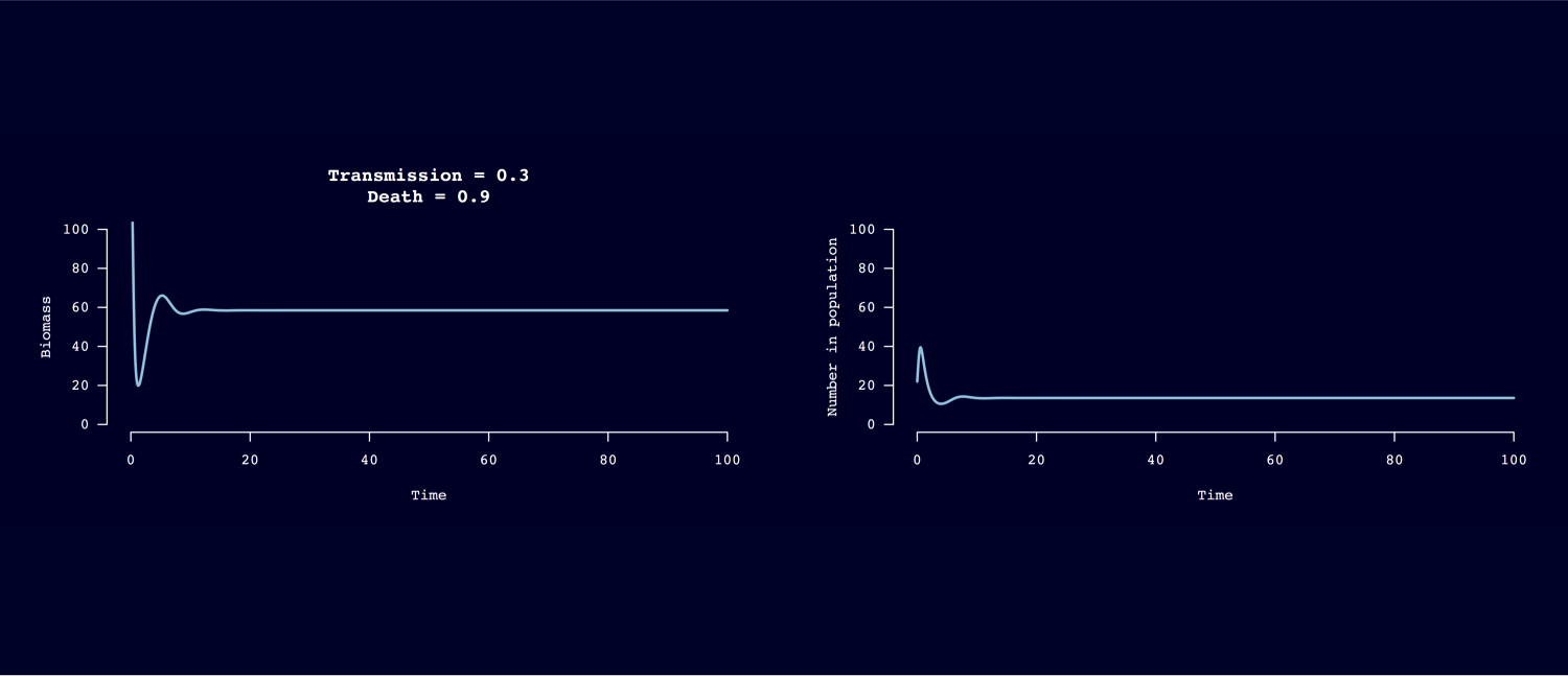
Header image: A 100-year model forecast of susceptible host biomass (left) and population density (right) under macroparasite infection with low transmission rate and high host mortality rate.